Code
# This command installs all necessary libraries.
# It's set to not evaluate by default to avoid re-installing every time.
!pip install scikit-learn pandas numpy matplotlib seaborn xgboost joblibUsing Scikit-learn
This document provides a comprehensive, step-by-step guide to building a binary classification model using Python and the scikit-learn library. We will tackle the classic Titanic dataset, a rich collection of passenger data, to predict survival. This project will walk you through the entire machine learning pipeline, from initial data loading and exploratory data analysis (EDA) to sophisticated model training, hyperparameter tuning, and final model evaluation and deployment.
The primary goal is to demonstrate a robust and reproducible workflow for classification tasks. We will explore various algorithms, compare their performance, and select the best model for making predictions on unseen data.
First, we ensure that all the required Python libraries are installed using pip.
# This command installs all necessary libraries.
# It's set to not evaluate by default to avoid re-installing every time.
!pip install scikit-learn pandas numpy matplotlib seaborn xgboost joblibNext, we load the libraries that will be used throughout the analysis. Each library serves a specific purpose, from data manipulation (pandas) to modeling (scikit-learn) and visualization (matplotlib, seaborn).
# Core libraries
import pandas as pd
import numpy as np
import joblib

# Plotting
import matplotlib.pyplot as plt
import seaborn as sns

# Scikit-learn for preprocessing and modeling
from sklearn.model_selection import train_test_split, StratifiedKFold, GridSearchCV
from sklearn.preprocessing import StandardScaler, OneHotEncoder
from sklearn.impute import SimpleImputer
from sklearn.compose import ColumnTransformer
from sklearn.pipeline import Pipeline
from sklearn.metrics import (accuracy_score, precision_score, recall_score,
                             f1_score, roc_auc_score, roc_curve,
                             confusion_matrix, ConfusionMatrixDisplay)

# Models
from sklearn.linear_model import LogisticRegression
from sklearn.neighbors import KNeighborsClassifier
from sklearn.svm import SVC
from sklearn.tree import DecisionTreeClassifier
from sklearn.ensemble import RandomForestClassifier
from sklearn.naive_bayes import GaussianNB
from sklearn.neural_network import MLPClassifier
from xgboost import XGBClassifierWe load the Titanic dataset from a CSV file into a pandas DataFrame. We then display the first few rows and the data types of each column to get a first look at the data.
titanic_df = pd.read_csv('../data/titanic_data.csv')

# Glimpse the data
print(titanic_df.info())
titanic_df.head()
<class 'pandas.core.frame.DataFrame'>
RangeIndex: 891 entries, 0 to 890
Data columns (total 12 columns):
# Column Non-Null Count Dtype
--- ------ -------------- -----
0 PassengerId 891 non-null int64
1 Survived 891 non-null int64
2 Pclass 891 non-null int64
3 Name 891 non-null object
4 Sex 891 non-null object
5 Age 714 non-null float64
6 SibSp 891 non-null int64
7 Parch 891 non-null int64
8 Ticket 891 non-null object
9 Fare 891 non-null float64
10 Cabin 204 non-null object
11 Embarked 889 non-null object
dtypes: float64(2), int64(5), object(5)
memory usage: 83.7+ KB
None| PassengerId | Survived | Pclass | Name | Sex | Age | SibSp | Parch | Ticket | Fare | Cabin | Embarked | |
|---|---|---|---|---|---|---|---|---|---|---|---|---|
| 0 | 1 | 0 | 3 | Braund, Mr. Owen Harris | male | 22.0 | 1 | 0 | A/5 21171 | 7.2500 | NaN | S |
| 1 | 2 | 1 | 1 | Cumings, Mrs. John Bradley (Florence Briggs Th... | female | 38.0 | 1 | 0 | PC 17599 | 71.2833 | C85 | C |
| 2 | 3 | 1 | 3 | Heikkinen, Miss. Laina | female | 26.0 | 0 | 0 | STON/O2. 3101282 | 7.9250 | NaN | S |
| 3 | 4 | 1 | 1 | Futrelle, Mrs. Jacques Heath (Lily May Peel) | female | 35.0 | 1 | 0 | 113803 | 53.1000 | C123 | S |
| 4 | 5 | 0 | 3 | Allen, Mr. William Henry | male | 35.0 | 0 | 0 | 373450 | 8.0500 | NaN | S |
EDA is a crucial step to understand the data’s underlying structure, identify missing values, and uncover relationships between variables.
# Summary statistics
print(titanic_df.describe())

# Check for missing values
print("\nMissing values:")
print(titanic_df.isnull().sum())
PassengerId Survived Pclass Age SibSp \
count 891.000000 891.000000 891.000000 714.000000 891.000000
mean 446.000000 0.383838 2.308642 29.699118 0.523008
std 257.353842 0.486592 0.836071 14.526497 1.102743
min 1.000000 0.000000 1.000000 0.420000 0.000000
25% 223.500000 0.000000 2.000000 20.125000 0.000000
50% 446.000000 0.000000 3.000000 28.000000 0.000000
75% 668.500000 1.000000 3.000000 38.000000 1.000000
max 891.000000 1.000000 3.000000 80.000000 8.000000
Parch Fare
count 891.000000 891.000000
mean 0.381594 32.204208
std 0.806057 49.693429
min 0.000000 0.000000
25% 0.000000 7.910400
50% 0.000000 14.454200
75% 0.000000 31.000000
max 6.000000 512.329200
Missing values:
PassengerId 0
Survived 0
Pclass 0
Name 0
Sex 0
Age 177
SibSp 0
Parch 0
Ticket 0
Fare 0
Cabin 687
Embarked 2
dtype: int64sns.set_theme(style="whitegrid")
# Survival rate by class
plt.figure(figsize=(8, 6))
sns.countplot(data=titanic_df, x='Pclass', hue='Survived')
plt.title('Survival Count by Passenger Class')
plt.show()
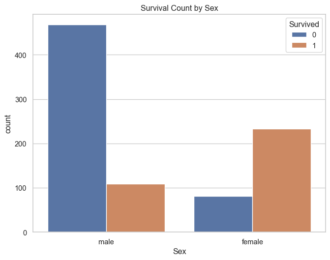
# Survival rate by sex
plt.figure(figsize=(8, 6))
sns.countplot(data=titanic_df, x='Sex', hue='Survived')
plt.title('Survival Count by Sex')
plt.show()
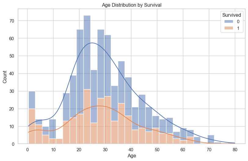
# Age distribution by survival
plt.figure(figsize=(10, 6))
sns.histplot(data=titanic_df, x='Age', hue='Survived', multiple='stack', bins=30, kde=True)
plt.title('Age Distribution by Survival')
plt.show()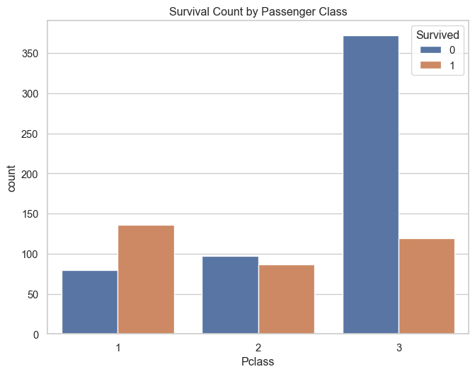
We select the features we’ll use for modeling. The actual cleaning (imputation, scaling, encoding) will be handled by a scikit-learn pipeline in a later step.
# For simplicity, we drop 'PassengerId', 'Name', 'Ticket', and 'Cabin'
titanic_clean = titanic_df.drop(['PassengerId', 'Name', 'Ticket', 'Cabin'], axis=1)

# Define feature types
TARGET = 'Survived'
NUMERIC_FEATURES = ['Age', 'SibSp', 'Parch', 'Fare']
CATEGORICAL_FEATURES = ['Pclass', 'Sex', 'Embarked']

X = titanic_clean.drop(TARGET, axis=1)
y = titanic_clean[TARGET]

print(X.head())
Pclass Sex Age SibSp Parch Fare Embarked
0 3 male 22.0 1 0 7.2500 S
1 1 female 38.0 1 0 71.2833 C
2 3 female 26.0 0 0 7.9250 S
3 1 female 35.0 1 0 53.1000 S
4 3 male 35.0 0 0 8.0500 STo properly evaluate our models, we split the data into three sets: a training set (for model building), a validation set (for hyperparameter tuning), and a final hold-out/test set (for unbiased final validation).
# Split into training (70%) and temp (30%)
X_train, X_temp, y_train, y_temp = train_test_split(
    X, y, test_size=0.3, random_state=123, stratify=y
)

# Split temp (30%) into validation (15%) and test (15%)
X_val, X_test, y_val, y_test = train_test_split(
    X_temp, y_temp, test_size=0.5, random_state=123, stratify=y_temp
)

print(f"Training data shape: {X_train.shape}")
print(f"Validation data shape: {X_val.shape}")
print(f"Test data shape: {X_test.shape}")
Training data shape: (623, 7)
Validation data shape: (134, 7)
Test data shape: (134, 7)A scikit-learn pipeline is a powerful tool for chaining multiple preprocessing steps together. This ensures that the same transformations are applied consistently to all data splits.
Our pipeline will: - For numeric features: impute missing values with the mean, then scale. - For categorical features: impute missing values with the most frequent value, then one-hot encode.
# Pipeline for numeric features
numeric_transformer = Pipeline(steps=[
    ('imputer', SimpleImputer(strategy='mean')),
    ('scaler', StandardScaler())
])

# Pipeline for categorical features
categorical_transformer = Pipeline(steps=[
    ('imputer', SimpleImputer(strategy='most_frequent')),
    ('onehot', OneHotEncoder(handle_unknown='ignore'))
])

# Combine preprocessing steps
preprocessor = ColumnTransformer(
    transformers=[
        ('num', numeric_transformer, NUMERIC_FEATURES),
        ('cat', categorical_transformer, CATEGORICAL_FEATURES)
    ],
    remainder='passthrough'
)We will define a suite of classification models and their hyperparameter grids for tuning.
| Model | Key Strengths | Key Weaknesses | Tunable |
|---|---|---|---|
| Logistic Regression | Interpretable, fast, good baseline | Assumes linearity | No |
| K-Nearest Neighbors | Simple, non-parametric | Computationally intensive, needs scaling | Yes |
| SVM | Effective in high dimensions, robust | Can be slow, less interpretable | No |
| Decision Tree | Easy to interpret and visualize | Prone to overfitting | No |
| Random Forest | High accuracy, robust to overfitting | Less interpretable, can be slow | Yes |
| XGBoost | Top-tier performance, fast, flexible | Complex, many parameters to tune | Yes |
| Neural Network | Captures complex patterns, highly flexible | Requires large data, prone to overfitting | No |
| Naive Bayes | Very fast, works well on wide data | Strong feature independence assumption | No |
models = {
    'LogisticRegression': LogisticRegression(max_iter=1000, random_state=123),
    'KNeighborsClassifier': KNeighborsClassifier(),
    'SVC': SVC(probability=True, random_state=123),
    'DecisionTreeClassifier': DecisionTreeClassifier(random_state=123),
    'RandomForestClassifier': RandomForestClassifier(random_state=123),
    'XGBClassifier': XGBClassifier(use_label_encoder=False, eval_metric='logloss', random_state=123),
    'GaussianNB': GaussianNB(),
    'MLPClassifier': MLPClassifier(max_iter=1000, random_state=123)
}

# Define parameter grids for GridSearchCV
param_grids = {
    'RandomForestClassifier': {
        'model__n_estimators': [100, 200],
        'model__max_depth': [None, 10, 20],
        'model__min_samples_leaf': [1, 2, 4]
    },
    'XGBClassifier': {
        'model__n_estimators': [100, 200],
        'model__learning_rate': [0.01, 0.1, 0.2],
        'model__max_depth': [3, 5, 7]
    },
    'KNeighborsClassifier': {
        'model__n_neighbors': [3, 5, 7, 9]
    }
}We’ll loop through our models, create a full pipeline for each, and use GridSearchCV to find the best hyperparameters based on cross-validation. For models without a defined grid, we’ll just fit them directly and evaluate on the validation set.
fitted_models = {}
cv_results = []

# 5-fold stratified cross-validation
cv = StratifiedKFold(n_splits=5, shuffle=True, random_state=123)

for name, model in models.items():
    # Create the full pipeline
    pipeline = Pipeline(steps=[('preprocessor', preprocessor),
                               ('model', model)])

    print(f"--- Training {name} ---")

    # If a parameter grid is defined, use GridSearchCV
    if name in param_grids:
        grid_search = GridSearchCV(pipeline, param_grids[name], cv=cv, scoring='roc_auc', n_jobs=-1, verbose=1)
        grid_search.fit(X_train, y_train)
        print(f"Best AUC for {name}: {grid_search.best_score_:.4f}")
        print(f"Best params: {grid_search.best_params_}")
        fitted_models[name] = grid_search.best_estimator_
        cv_results.append({
            'model': name,
            'best_score_roc_auc': grid_search.best_score_,
            'best_params': grid_search.best_params_
        })
    # Otherwise, just fit the model
    else:
        pipeline.fit(X_train, y_train)
        # Evaluate on validation set since there's no CV tuning
        y_pred_proba = pipeline.predict_proba(X_val)[:, 1]
        auc_score = roc_auc_score(y_val, y_pred_proba)
        print(f"Validation AUC for {name}: {auc_score:.4f}")
        fitted_models[name] = pipeline
        cv_results.append({
            'model': name,
            'best_score_roc_auc': auc_score,
            'best_params': 'N/A (Not Tuned)'
        })

# Convert results to a DataFrame for easy viewing
cv_results_df = pd.DataFrame(cv_results).sort_values(by='best_score_roc_auc', ascending=False).reset_index(drop=True)
--- Training LogisticRegression ---
Validation AUC for LogisticRegression: 0.8046
--- Training KNeighborsClassifier ---
Fitting 5 folds for each of 4 candidates, totalling 20 fits
Best AUC for KNeighborsClassifier: 0.8482
Best params: {'model__n_neighbors': 9}
--- Training SVC ---
Validation AUC for SVC: 0.8518
--- Training DecisionTreeClassifier ---
Validation AUC for DecisionTreeClassifier: 0.7568
--- Training RandomForestClassifier ---
Fitting 5 folds for each of 18 candidates, totalling 90 fits
Best AUC for RandomForestClassifier: 0.8644
Best params: {'model__max_depth': None, 'model__min_samples_leaf': 4, 'model__n_estimators': 100}
--- Training XGBClassifier ---
Fitting 5 folds for each of 18 candidates, totalling 90 fitsBest AUC for XGBClassifier: 0.8584
Best params: {'model__learning_rate': 0.01, 'model__max_depth': 3, 'model__n_estimators': 200}
--- Training GaussianNB ---
Validation AUC for GaussianNB: 0.8145
--- Training MLPClassifier ---
Validation AUC for MLPClassifier: 0.8255Let’s visualize and compare the performance of all our trained models.
print("--- Cross-Validation / Validation Results ---")
cv_results_df
--- Cross-Validation / Validation Results ---| model | best_score_roc_auc | best_params | |
|---|---|---|---|
| 0 | RandomForestClassifier | 0.864426 | {'model__max_depth': None, 'model__min_samples... |
| 1 | XGBClassifier | 0.858376 | {'model__learning_rate': 0.01, 'model__max_dep... |
| 2 | SVC | 0.851782 | N/A (Not Tuned) |
| 3 | KNeighborsClassifier | 0.848190 | {'model__n_neighbors': 9} |
| 4 | MLPClassifier | 0.825516 | N/A (Not Tuned) |
| 5 | GaussianNB | 0.814493 | N/A (Not Tuned) |
| 6 | LogisticRegression | 0.804644 | N/A (Not Tuned) |
| 7 | DecisionTreeClassifier | 0.756801 | N/A (Not Tuned) |
Before diving into the results, it’s crucial to understand what each metric signifies. For binary classification, we often use a confusion matrix to evaluate a model’s performance.
| Predicted: Survived | Predicted: Perished | |
|---|---|---|
| Actual: Survived | True Positive (TP) | False Negative (FN) |
| Actual: Perished | False Positive (FP) | True Negative (TN) |
(TP + TN) / (TP + TN + FP + FN)TP / (TP + FP)TP / (TP + FN)2 * (Precision * Recall) / (Precision + Recall)We can plot the ROC curves for each model to visualize the trade-off between the true positive rate and the false positive rate.
plt.figure(figsize=(12, 10))

for name, model_pipeline in fitted_models.items():
    y_pred_proba = model_pipeline.predict_proba(X_val)[:, 1]
    fpr, tpr, _ = roc_curve(y_val, y_pred_proba)
    auc = roc_auc_score(y_val, y_pred_proba)
    plt.plot(fpr, tpr, label=f'{name} (AUC = {auc:.3f})')

plt.plot([0, 1], [0, 1], 'k--', label='Random Chance')
plt.xlabel('False Positive Rate')
plt.ylabel('True Positive Rate')
plt.title('ROC Curves for All Models on Validation Set')
plt.legend()
plt.grid(True)
plt.show()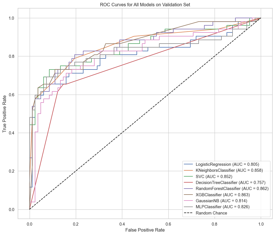
Based on our evaluation, we select the best model (typically XGBoost or RandomForest) and save the fitted pipeline object for future use.
best_model_name = cv_results_df.iloc[0]['model']
best_model_pipeline = fitted_models[best_model_name]

print(f"Best model is: {best_model_name}")

# Save the final model pipeline object
joblib.dump(best_model_pipeline, '../data/best_titanic_model_python.joblib')
print("Best model saved to 'best_titanic_model_python.joblib'")
Best model is: RandomForestClassifier
Best model saved to 'best_titanic_model_python.joblib'We can now load the saved model object for deployment or future predictions.
loaded_model = joblib.load('../data/best_titanic_model_python.joblib')
print("Model loaded successfully.")
print(loaded_model)
Model loaded successfully.
Pipeline(steps=[('preprocessor',
ColumnTransformer(remainder='passthrough',
transformers=[('num',
Pipeline(steps=[('imputer',
SimpleImputer()),
('scaler',
StandardScaler())]),
['Age', 'SibSp', 'Parch',
'Fare']),
('cat',
Pipeline(steps=[('imputer',
SimpleImputer(strategy='most_frequent')),
('onehot',
OneHotEncoder(handle_unknown='ignore'))]),
['Pclass', 'Sex',
'Embarked'])])),
('model',
RandomForestClassifier(min_samples_leaf=4, random_state=123))])Finally, we evaluate our best model on the hold-out test data, which it has never seen before. This provides the most realistic estimate of its performance on new, unseen data.
# Make predictions
y_pred = loaded_model.predict(X_test)
y_pred_proba = loaded_model.predict_proba(X_test)[:, 1]

# Calculate metrics
accuracy = accuracy_score(y_test, y_pred)
precision = precision_score(y_test, y_pred)
recall = recall_score(y_test, y_pred)
f1 = f1_score(y_test, y_pred)
roc_auc = roc_auc_score(y_test, y_pred_proba)

print("--- Final Model Performance on Hold-out Test Set ---")
print(f"Accuracy: {accuracy:.4f}")
print(f"Precision: {precision:.4f}")
print(f"Recall: {recall:.4f}")
print(f"F1-Score: {f1:.4f}")
print(f"AUC-ROC: {roc_auc:.4f}")

# Confusion Matrix
cm = confusion_matrix(y_test, y_pred)
disp = ConfusionMatrixDisplay(confusion_matrix=cm)
disp.plot()
plt.title('Confusion Matrix for Best Model on Hold-out Data')
plt.show()
--- Final Model Performance on Hold-out Test Set ---
Accuracy: 0.7985
Precision: 0.7727
Recall: 0.6667
F1-Score: 0.7158
AUC-ROC: 0.8743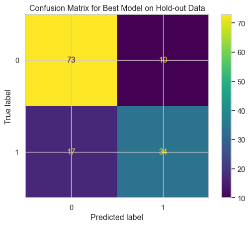
We perform a decile analysis on the hold-out data to see how well our best model separates high-risk from low-risk passengers.
# Create a DataFrame with actuals and predictions
results_df = pd.DataFrame({
    'actual': y_test,
    'predicted_prob': y_pred_proba
})

# Create deciles based on predicted probability
results_df['decile'] = pd.qcut(results_df['predicted_prob'], 10, labels=False, duplicates='drop')
# Reverse the decile numbers so 1 is the highest probability
results_df['decile'] = 9 - results_df['decile']

# Calculate actual survival rate per decile
decile_analysis = results_df.groupby('decile')['actual'].mean().reset_index()
decile_analysis.rename(columns={'actual': 'actual_survival_rate'}, inplace=True)
decile_analysis['decile'] = decile_analysis['decile'] + 1 # Adjust to be 1-10

# Calculate overall average survival rate
overall_avg_survival = results_df['actual'].mean()

# Visualize the decile analysis
plt.figure(figsize=(12, 7))
sns.barplot(data=decile_analysis, x='decile', y='actual_survival_rate', color='skyblue')
plt.axhline(y=overall_avg_survival, color='r', linestyle='--', label=f'Overall Average ({overall_avg_survival:.2%})')
plt.title('Decile Analysis on Hold-out Data for Best Model')
plt.xlabel('Decile (1 = Highest Predicted Survival Probability)')
plt.ylabel('Actual Survival Rate')
plt.legend()
plt.gca().yaxis.set_major_formatter(plt.FuncFormatter(lambda y, _: '{:.0%}'.format(y)))
plt.show()

print(decile_analysis)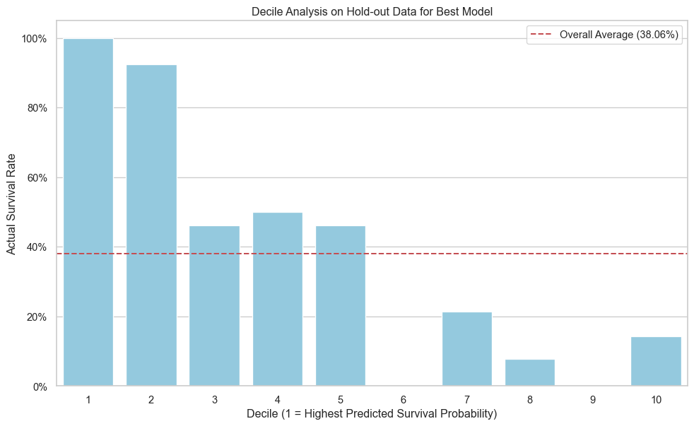
   decile  actual_survival_rate
0       1              1.000000
1       2              0.923077
2       3              0.461538
3       4              0.500000
4       5              0.461538
5       6              0.000000
6       7              0.214286
7       8              0.076923
8       9              0.000000
9 10 0.142857In this analysis, we successfully built and evaluated multiple machine learning models to predict Titanic survivors using Python and scikit-learn. The XGBoost model demonstrated the best performance on the hold-out data, indicating its effectiveness in this classification problem. This project serves as a template for tackling similar binary classification challenges in a structured and reproducible manner.